TensorFlowのバージョン指定(Google Colaboratory)
少し前からColaboでTensorFlow使おうとするとエラーになったのでメモ (バージョンが変わったのだろう)
- バージョン1.14指定
%%time
!pip uninstall -y tensorflow
!pip install tensorflow-gpu==1.14.
2分くらいかかる、そのあと確認
import tensorflow as tf
print(tf.__version__)
統計検定
業務で検定をする機会があったので備忘録としてメモ
統計検定の手順
- 事前に以下を決める
- 検出力
- 効果量
- これ求めるの大変だったりするのかも
- 顧客とも事前に認識合わせておく必要ありと思われる
- 有意水準
- サンプルサイズ
- 検定手法を決める
検定手法
- パラメトリック
- t検定(ステューデント、ウェルチ)
- ノンパラメトリック
- ウィルコクソン
- 並び替え
- DID(差分の差分法)
- 以下を考慮する必要がある?
- 並行トレンド仮定
- 共通ショック仮定
- 以下を考慮する必要がある?
- その他
- 傾向スコアも使える?
ワード
- 検出力
- 効果量
- コーエンの標本効果量(Cohen's d)
- ヘッジズの効果量(Hedges' g)
- 量的変数の相関の強さならピアソンの積率相関係数
- 大きく設定
- 検出しやすくなり、必要なサンプルサイズは少なくなる
- 小さく設定
- ノイズでも効果ありと判断する場合がある
- 上記を考慮して効果量設定する必要あり
参考
kaggle walmart EDA (引用)
- 元のnotebook
- インポート
- データ
- 予測するものは何か?
- 一つの商品のデータを可視化
- 売上データと日付を結合
- 期間単位の売上
- さらに複数の商品の売上をみる
- カテゴリ別の商品数
- カテゴリ別の売上推移
- 販売中の商品割合
- 店舗ごと売上
- 店舗ごとの7日間の平均売上の推移
- 売上ヒートマップカレンダー
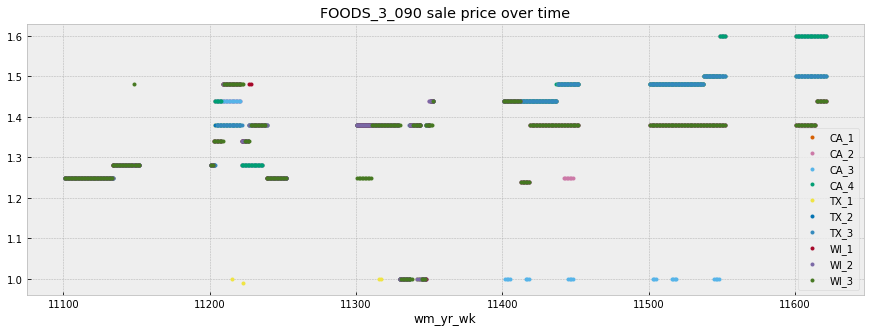
- 販売価格
- 単純な予測
元のnotebook
https://www.kaggle.com/robikscube/m5-forecasting-starter-data-exploration
インポート
import pandas as pd
import numpy as np
import matplotlib.pylab as plt
import seaborn as sns
from itertools import cycle
pd.set_option('max_columns', 50)
plt.style.use('bmh') # matplotlibのスタイルを変える
color_pal = plt.rcParams['axes.prop_cycle'].by_key()['color'] # 11種類の色を指定
color_cycle = cycle(plt.rcParams['axes.prop_cycle'].by_key()['color']) # それをサイクルでぐるぐる回して使う?
データ
calendar.csv- 日付情報sales_train_validation.csv- 1日毎の売上が商品毎に入っている(1913日間)sample_submission.csv- 提出用ファイルのサンプルsell_prices.csv- 商品販売価格が商品毎、日毎に入っているsales_train_evaluation.csv- (現状まだ利用できない)1914日目〜1941日目の売上データ
%%time
# データ読み込み
INPUT_DIR = 'input/'
cal = pd.read_csv(INPUT_DIR + "calendar.csv")
stv = pd.read_csv(INPUT_DIR + "sales_train_validation.csv")
ss = pd.read_csv(INPUT_DIR + "sample_submission.csv")
sellp = pd.read_csv(INPUT_DIR + "sell_prices.csv")
CPU times: user 7.26 s, sys: 633 ms, total: 7.9 s
Wall time: 8.27 s
print(cal.shape)
print(stv.shape)
print(ss.shape)
print(sellp.shape)
(1969, 14)
(30490, 1919)
(60980, 29)
(6841121, 4)
予測するものは何か?
- 28日間の日毎の商品ごとの売上
- sample submissionを見れば何をどう予測すべきかがわかる
- データは一行が一商品を表しており、店舗の州、商品カテゴリ、IDがわかる
ss.head()
| id | F1 | F2 | F3 | F4 | F5 | F6 | F7 | F8 | F9 | F10 | F11 | F12 | F13 | F14 | F15 | F16 | F17 | F18 | F19 | F20 | F21 | F22 | F23 | F24 | F25 | F26 | F27 | F28 | |
|---|---|---|---|---|---|---|---|---|---|---|---|---|---|---|---|---|---|---|---|---|---|---|---|---|---|---|---|---|---|
| 0 | HOBBIES_1_001_CA_1_validation | 0 | 0 | 0 | 0 | 0 | 0 | 0 | 0 | 0 | 0 | 0 | 0 | 0 | 0 | 0 | 0 | 0 | 0 | 0 | 0 | 0 | 0 | 0 | 0 | 0 | 0 | 0 | 0 |
| 1 | HOBBIES_1_002_CA_1_validation | 0 | 0 | 0 | 0 | 0 | 0 | 0 | 0 | 0 | 0 | 0 | 0 | 0 | 0 | 0 | 0 | 0 | 0 | 0 | 0 | 0 | 0 | 0 | 0 | 0 | 0 | 0 | 0 |
| 2 | HOBBIES_1_003_CA_1_validation | 0 | 0 | 0 | 0 | 0 | 0 | 0 | 0 | 0 | 0 | 0 | 0 | 0 | 0 | 0 | 0 | 0 | 0 | 0 | 0 | 0 | 0 | 0 | 0 | 0 | 0 | 0 | 0 |
| 3 | HOBBIES_1_004_CA_1_validation | 0 | 0 | 0 | 0 | 0 | 0 | 0 | 0 | 0 | 0 | 0 | 0 | 0 | 0 | 0 | 0 | 0 | 0 | 0 | 0 | 0 | 0 | 0 | 0 | 0 | 0 | 0 | 0 |
| 4 | HOBBIES_1_005_CA_1_validation | 0 | 0 | 0 | 0 | 0 | 0 | 0 | 0 | 0 | 0 | 0 | 0 | 0 | 0 | 0 | 0 | 0 | 0 | 0 | 0 | 0 | 0 | 0 | 0 | 0 | 0 | 0 | 0 |
stv.head()
| id | item_id | dept_id | cat_id | store_id | state_id | d_1 | d_2 | d_3 | d_4 | d_5 | d_6 | d_7 | d_8 | d_9 | d_10 | d_11 | d_12 | d_13 | d_14 | d_15 | d_16 | d_17 | d_18 | d_19 | ... | d_1889 | d_1890 | d_1891 | d_1892 | d_1893 | d_1894 | d_1895 | d_1896 | d_1897 | d_1898 | d_1899 | d_1900 | d_1901 | d_1902 | d_1903 | d_1904 | d_1905 | d_1906 | d_1907 | d_1908 | d_1909 | d_1910 | d_1911 | d_1912 | d_1913 | |
|---|---|---|---|---|---|---|---|---|---|---|---|---|---|---|---|---|---|---|---|---|---|---|---|---|---|---|---|---|---|---|---|---|---|---|---|---|---|---|---|---|---|---|---|---|---|---|---|---|---|---|---|
| 0 | HOBBIES_1_001_CA_1_validation | HOBBIES_1_001 | HOBBIES_1 | HOBBIES | CA_1 | CA | 0 | 0 | 0 | 0 | 0 | 0 | 0 | 0 | 0 | 0 | 0 | 0 | 0 | 0 | 0 | 0 | 0 | 0 | 0 | ... | 0 | 0 | 0 | 1 | 0 | 4 | 2 | 3 | 0 | 1 | 2 | 0 | 0 | 0 | 1 | 1 | 3 | 0 | 1 | 1 | 1 | 3 | 0 | 1 | 1 |
| 1 | HOBBIES_1_002_CA_1_validation | HOBBIES_1_002 | HOBBIES_1 | HOBBIES | CA_1 | CA | 0 | 0 | 0 | 0 | 0 | 0 | 0 | 0 | 0 | 0 | 0 | 0 | 0 | 0 | 0 | 0 | 0 | 0 | 0 | ... | 0 | 0 | 0 | 0 | 0 | 0 | 0 | 0 | 0 | 0 | 0 | 0 | 0 | 0 | 0 | 0 | 0 | 0 | 0 | 0 | 1 | 0 | 0 | 0 | 0 |
| 2 | HOBBIES_1_003_CA_1_validation | HOBBIES_1_003 | HOBBIES_1 | HOBBIES | CA_1 | CA | 0 | 0 | 0 | 0 | 0 | 0 | 0 | 0 | 0 | 0 | 0 | 0 | 0 | 0 | 0 | 0 | 0 | 0 | 0 | ... | 0 | 0 | 0 | 1 | 0 | 0 | 0 | 1 | 0 | 0 | 0 | 0 | 0 | 1 | 2 | 2 | 1 | 2 | 1 | 1 | 1 | 0 | 1 | 1 | 1 |
| 3 | HOBBIES_1_004_CA_1_validation | HOBBIES_1_004 | HOBBIES_1 | HOBBIES | CA_1 | CA | 0 | 0 | 0 | 0 | 0 | 0 | 0 | 0 | 0 | 0 | 0 | 0 | 0 | 0 | 0 | 0 | 0 | 0 | 0 | ... | 0 | 3 | 1 | 2 | 1 | 3 | 1 | 0 | 2 | 5 | 4 | 2 | 0 | 3 | 0 | 1 | 0 | 5 | 4 | 1 | 0 | 1 | 3 | 7 | 2 |
| 4 | HOBBIES_1_005_CA_1_validation | HOBBIES_1_005 | HOBBIES_1 | HOBBIES | CA_1 | CA | 0 | 0 | 0 | 0 | 0 | 0 | 0 | 0 | 0 | 0 | 0 | 0 | 0 | 0 | 0 | 0 | 0 | 0 | 0 | ... | 4 | 0 | 1 | 4 | 0 | 1 | 0 | 1 | 0 | 1 | 1 | 2 | 0 | 1 | 1 | 2 | 1 | 1 | 0 | 1 | 1 | 2 | 2 | 2 | 4 |
5 rows × 1919 columns
一つの商品のデータを可視化
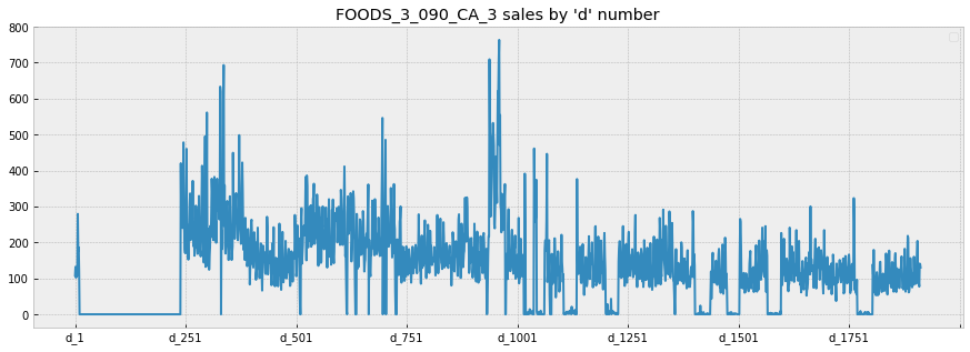
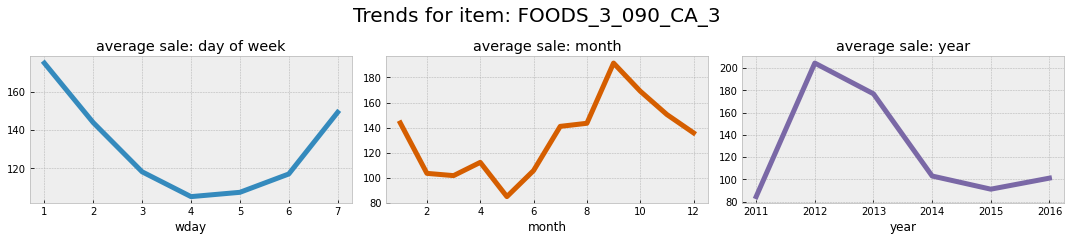
FOODS_3_090_CA_3_validationはよく売れている商品?- 取り扱いのない日はがあるようだ
d_cols = [c for c in stv.columns if "d_" in c] # sales data columns
len(d_cols)

stv.loc[stv["id"] == "FOODS_3_090_CA_3_validation"] \
    .set_index("id")[d_cols] \
    .T \
    .plot(figsize=(15, 5),
          title="FOODS_3_090_CA_3 sales by 'd' number",
          color=next(color_cycle)) # next():イテレータの先頭要素を取得するために用いる関数
plt.legend("")
plt.show()

売上データと日付を結合
# 曜日や他の州等結構削っている
cal[['d','date','event_name_1','event_name_2',
     'event_type_1','event_type_2', 'snap_CA']].head()
| d | date | event_name_1 | event_name_2 | event_type_1 | event_type_2 | snap_CA | |
|---|---|---|---|---|---|---|---|
| 0 | d_1 | 2011-01-29 | NaN | NaN | NaN | NaN | 0 |
| 1 | d_2 | 2011-01-30 | NaN | NaN | NaN | NaN | 0 |
| 2 | d_3 | 2011-01-31 | NaN | NaN | NaN | NaN | 0 |
| 3 | d_4 | 2011-02-01 | NaN | NaN | NaN | NaN | 1 |
| 4 | d_5 | 2011-02-02 | NaN | NaN | NaN | NaN | 1 |
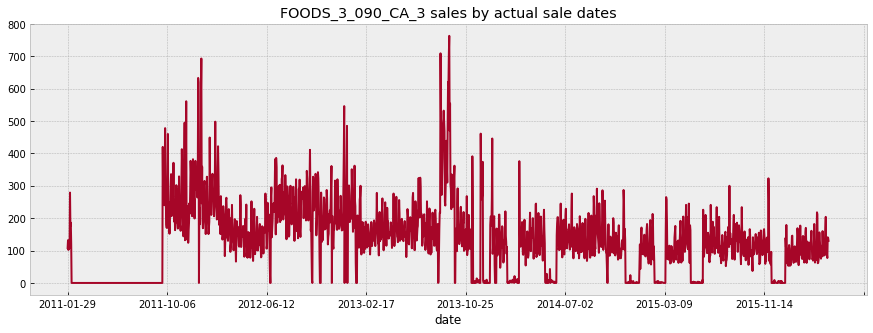
# calendarの日付をstvにmerge
example = stv.loc[stv["id"] == 'FOODS_3_090_CA_3_validation'][d_cols].T
example = example.rename(columns={8412:"FOODS_3_090_CA_3"})
example = example.reset_index().rename(columns={"index": "d"})
example = example.merge(cal, how="left", validate="1:1") # validate="1:1" →キーが1:1で一意でなければerrorをはく、keyは自動で判定している?
example.set_index("date")["FOODS_3_090_CA_3"] \
    .plot(figsize=(15, 5),
          color=next(color_cycle),
          title="FOODS_3_090_CA_3 sales by actual sale dates")
plt.show()

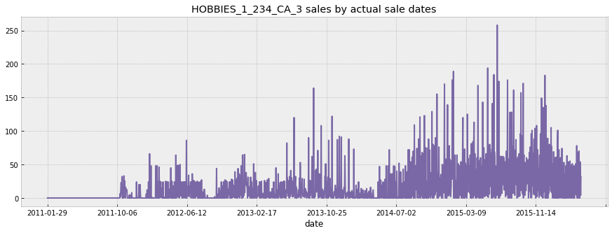
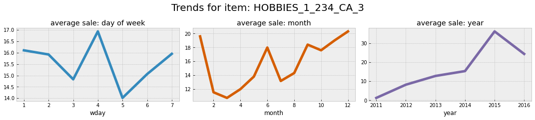
# 別の商品でも可視化(ホビー)
example2 = stv.loc[stv["id"] == "HOBBIES_1_234_CA_3_validation"][d_cols].T
example2 = example2.rename(columns={6324:"HOBBIES_1_234_CA_3"})
example2 = example2.reset_index().rename(columns={"index": "d"})
example2 = example2.merge(cal, how="left", validate="1:1")

example2.set_index("date")["HOBBIES_1_234_CA_3"] \
    .plot(figsize=(15, 5),
          color=next(color_cycle),
          title="HOBBIES_1_234_CA_3 sales by actual sale dates")
plt.show()

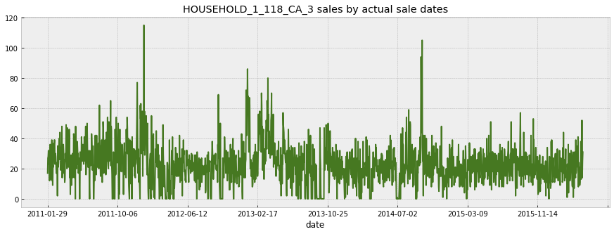
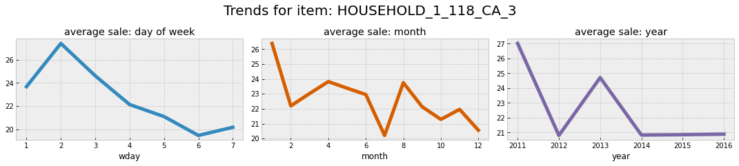
# 別の商品でも可視化(ハウスホールド、日用品?)
example3 = stv.loc[stv["id"] == "HOUSEHOLD_1_118_CA_3_validation"][d_cols].T
example3 = example3.rename(columns={6776:"HOUSEHOLD_1_118_CA_3"})
example3 = example3.reset_index().rename(columns={"index": "d"})
example3 = example3.merge(cal, how="left", validate="1:1")

example3.set_index("date")["HOUSEHOLD_1_118_CA_3"] \
    .plot(figsize=(15, 5),
          color=next(color_cycle),
          title="HOUSEHOLD_1_118_CA_3 sales by actual sale dates")
plt.show()

期間単位の売上
- 曜日
- 月
- 年
example["wday"].unique()
array([1, 2, 3, 4, 5, 6, 7])
example.head(2)
| d | FOODS_3_090_CA_3 | date | wm_yr_wk | weekday | wday | month | year | event_name_1 | event_type_1 | event_name_2 | event_type_2 | snap_CA | snap_TX | snap_WI | |
|---|---|---|---|---|---|---|---|---|---|---|---|---|---|---|---|
| 0 | d_1 | 108 | 2011-01-29 | 11101 | Saturday | 1 | 1 | 2011 | NaN | NaN | NaN | NaN | 0 | 0 | 0 |
| 1 | d_2 | 132 | 2011-01-30 | 11101 | Sunday | 2 | 1 | 2011 | NaN | NaN | NaN | NaN | 0 | 0 | 0 |
# food,hobbie,householdの1つずつのサンプルで売上状況を確認
# 曜日、月、年でみる
examples = ['FOODS_3_090_CA_3','HOBBIES_1_234_CA_3','HOUSEHOLD_1_118_CA_3']
# 3つのデータフレームをリストに格納
example_df = [example, example2, example3]

for i in [0, 1, 2]:
    fig, (ax1, ax2, ax3) = plt.subplots(1, 3, figsize=(15, 3)) # ax1-3で3行?、subplot1-3で3列?
    # 1列目、曜日(1:土曜日、2:日曜日、と続く)
    example_df[i].groupby("wday").mean()[examples[i]] \
        .plot(kind="line",
              title="average sale: day of week",
              lw=5, # 線の太さ
              color=color_pal[0],
              ax=ax1) # 1行目
    # 2列目、月
    example_df[i].groupby("month").mean()[examples[i]] \
        .plot(kind="line",
              title="average sale: month",
              lw=5, # 線の太さ
              color=color_pal[4],
              ax=ax2) # 2行目
    # 3列目、年
    example_df[i].groupby("year").mean()[examples[i]] \
        .plot(kind="line",
              title="average sale: year",
              lw=5, # 線の太さ
              color=color_pal[2],
              ax=ax3) # 3行目
    # 商品ごとのタイトル
    fig.suptitle(f"Trends for item: {examples[i]}",
                 size=20,
                 y=1.1)
    plt.tight_layout() # グラフの位置やサイズが自動で調整される
    plt.show()



さらに複数の商品の売上をみる
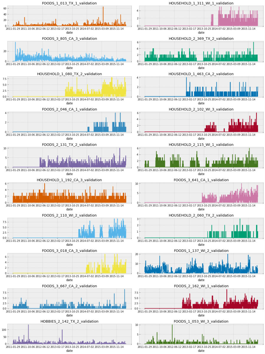
# インデックスが日付、カラムがサンプル商品20品目の売上データフレーム作成

# .sampleは重複なしの非復元抽出
# [d_cols]でカラムを1913日の売上データに絞る
# calendarのインデックスをd_1,d_2・・・とし、カラムdateのみのデータと結合
# left_index=True:leftのデータフレームの行ラベルを結合のキーとして用いる
# rightのデータフレームの行ラベルを結合のキーとして用いる

twenty_examples = stv.sample(20, random_state=529) \
    .set_index("id")[d_cols] \
    .T \
    .merge(cal.set_index("d")["date"],
           left_index=True,
           right_index=True,
           validate="1:1") \
    .set_index("date")
twenty_examples.head(3)
| FOODS_1_013_TX_1_validation | HOUSEHOLD_1_311_WI_1_validation | FOODS_3_805_CA_3_validation | HOUSEHOLD_2_369_TX_2_validation | HOUSEHOLD_1_080_TX_2_validation | HOUSEHOLD_1_463_CA_2_validation | FOODS_2_046_CA_1_validation | HOUSEHOLD_2_102_WI_3_validation | FOODS_2_131_TX_2_validation | HOUSEHOLD_2_115_WI_1_validation | HOUSEHOLD_1_192_CA_3_validation | FOODS_3_641_CA_1_validation | FOODS_2_110_WI_2_validation | HOUSEHOLD_2_060_TX_2_validation | FOODS_3_018_CA_3_validation | FOODS_1_137_WI_2_validation | FOODS_3_667_CA_2_validation | FOODS_2_162_WI_1_validation | HOBBIES_2_142_TX_2_validation | FOODS_1_053_WI_3_validation | |
|---|---|---|---|---|---|---|---|---|---|---|---|---|---|---|---|---|---|---|---|---|
| date | ||||||||||||||||||||
| 2011-01-29 | 0 | 0 | 0 | 0 | 0 | 0 | 0 | 0 | 0 | 0 | 0 | 0 | 0 | 0 | 0 | 6 | 1 | 0 | 1 | 0 |
| 2011-01-30 | 0 | 0 | 0 | 1 | 0 | 0 | 0 | 0 | 0 | 0 | 0 | 0 | 0 | 0 | 0 | 1 | 0 | 0 | 2 | 0 |
| 2011-01-31 | 0 | 0 | 0 | 3 | 0 | 0 | 0 | 0 | 0 | 0 | 2 | 0 | 0 | 0 | 0 | 6 | 0 | 0 | 0 | 0 |
fig, axs = plt.subplots(10, 2, figsize=(15, 20)) # 10行2列
axs = axs.flatten() # 10行2列を、20行に変換?
ax_idx = 0
for item in twenty_examples.columns:
    twenty_examples[item].plot(title=item,
                               color=next(color_cycle),
                               ax=axs[ax_idx]) # subplotsの10行列のどこに入るか指定
    ax_idx += 1
plt.tight_layout()
plt.show()

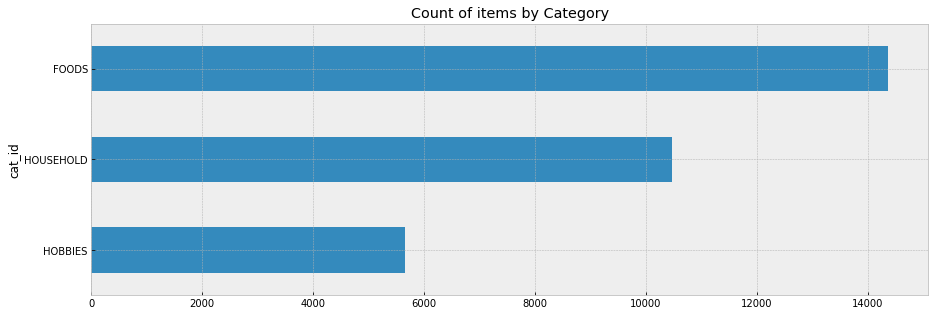
カテゴリ別の商品数
- HOBBIES
- HOUSEHOLD
- FOODS
stv['cat_id'].unique()
array(['HOBBIES', 'HOUSEHOLD', 'FOODS'], dtype=object)
stv.groupby("cat_id").count()["id"] \
    .sort_values() \
    .plot(kind="barh", figsize=(15, 5), title="Count of items by Category")
plt.show()

カテゴリ別の売上推移
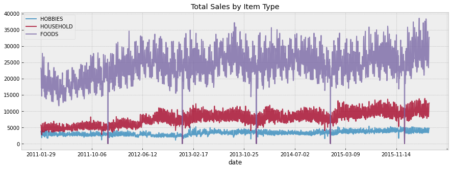
past_sales = stv.set_index("id")[d_cols] \
    .T \
    .merge(cal.set_index("d")["date"],
           left_index=True,
           right_index=True,
           validate="1:1") \
    .set_index("date")

# カテゴリ毎に1日の売上を合計してプロット
for i in stv["cat_id"].unique():
    items_col = [c for c in past_sales.columns if i in c]
    past_sales[items_col] \
        .sum(axis=1) \
        .plot(figsize=(15, 5),
              alpha=0.8,
              title="Total Sales by Item Type")
plt.legend(stv["cat_id"].unique())
plt.show()

販売中の商品割合
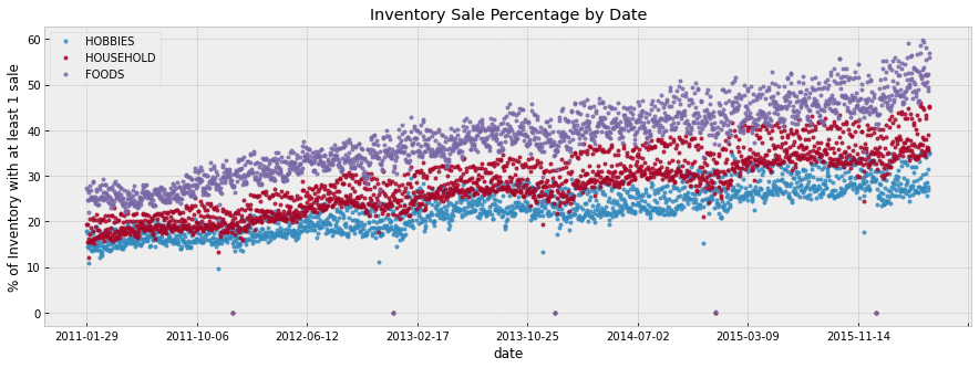
- カテゴリ別の売上が0でない商品割合
- 徐々に割合が上昇しており、期初は10-30%に対して、最終は20-60%となっている
past_sales_clipped = past_sales.clip(0, 1) # 売上を0or1に変換
for i in stv['cat_id'].unique():
    items_col = [c for c in past_sales.columns if i in c]
    (past_sales_clipped[items_col] \
        .mean(axis=1) * 100) \
        .plot(figsize=(15, 5),
              alpha=0.8,
              title='Inventory Sale Percentage by Date',
              style='.')
plt.ylabel('% of Inventory with at least 1 sale')
plt.legend(stv['cat_id'].unique())
plt.show()

店舗ごと売上
# ストアのリスト
store_list = sellp['store_id'].unique()

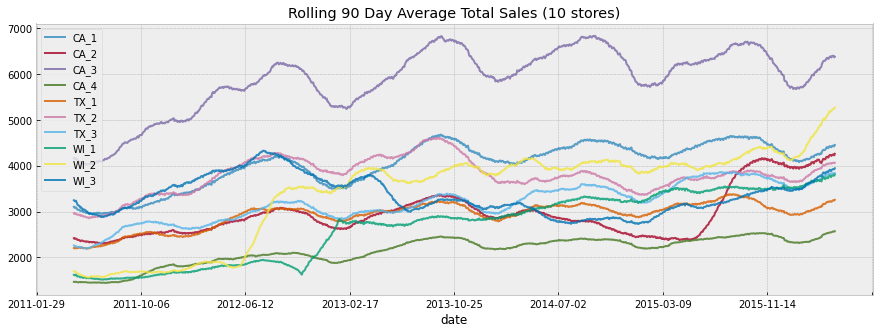
# ストア毎の90日間の平均売上の推移
for s in store_list:
    store_items = [c for c in past_sales.columns if s in c]
    past_sales[store_items] \
        .sum(axis=1) \
        .rolling(90).mean() \
        .plot(figsize=(15, 5),
              alpha=0.8,
              title='Rolling 90 Day Average Total Sales (10 stores)')
plt.legend(store_list)
plt.show()

店舗ごとの7日間の平均売上の推移
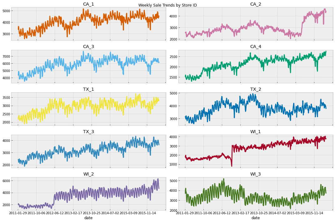
# 店舗により途中でトレンドに変化があるのが分かる
# 増加している店、減少している店
fig, axes = plt.subplots(5, 2, figsize=(15, 10), sharex=True) # sharex=True:X軸を共有
axes = axes.flatten()
ax_idx = 0
for s in store_list:
    store_items = [c for c in past_sales.columns if s in c]
    past_sales[store_items] \
        .sum(axis=1) \
        .rolling(7).mean() \
        .plot(alpha=1,
              ax=axes[ax_idx],
              title=s,
              lw=3,
              color=next(color_cycle))
    ax_idx += 1
# plt.legend(store_list)
plt.suptitle('Weekly Sale Trends by Store ID')
plt.tight_layout()
plt.show()

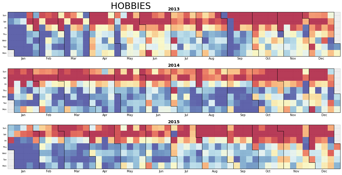
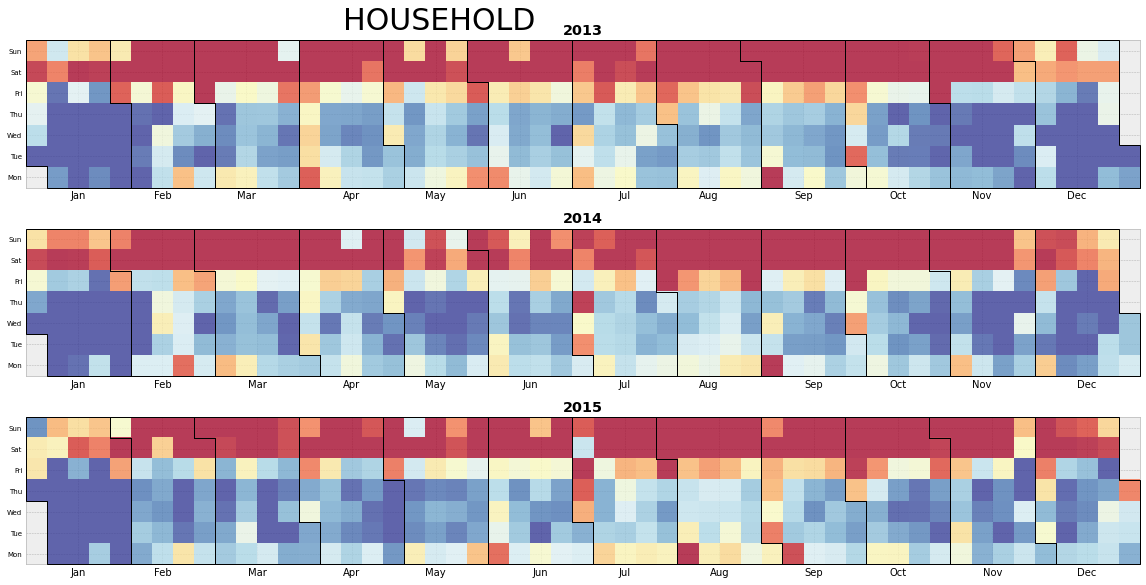
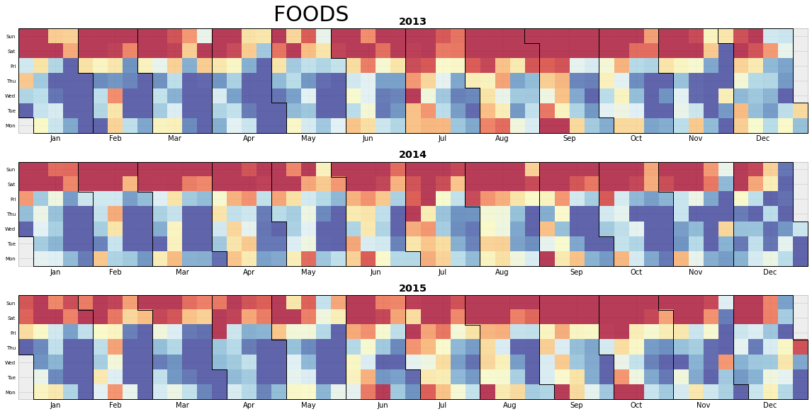
売上ヒートマップカレンダー
# ----------------------------------------------------------------------------
# Author:  Nicolas P. Rougier
# License: BSD
# ----------------------------------------------------------------------------
import numpy as np
import matplotlib.pyplot as plt
from matplotlib.patches import Polygon
from datetime import datetime
from dateutil.relativedelta import relativedelta

def calmap(ax, year, data):
    ax.tick_params('x', length=0, labelsize="medium", which='major')
    ax.tick_params('y', length=0, labelsize="x-small", which='major')

    # Month borders
    xticks, labels = [], []
    start = datetime(year,1,1).weekday() # weekday():月曜日が0で日曜日が6の整数値を得る
    for month in range(1,13):
        first = datetime(year, month, 1)
        last = first + relativedelta(months=1, days=-1) # 月末日の取得(1ヶ月加算して、1日マイナスするっぽい)

        y0 = first.weekday()
        y1 = last.weekday()
        x0 = (int(first.strftime("%j"))+start-1)//7 # strftime:日付を文字列に変換、%j : 0埋めした10進数で表記した年中の日にち(正月が'001')
        x1 = (int(last.strftime("%j"))+start-1)//7 # 年初から第何周目かを算出している?

        P = [ (x0,   y0), (x0,    7),  (x1,   7),
              (x1,   y1+1), (x1+1,  y1+1), (x1+1, 0),
              (x0+1,  0), (x0+1,  y0) ]
        xticks.append(x0 +(x1-x0+1)/2)
        labels.append(first.strftime("%b"))
        poly = Polygon(P, edgecolor="black", facecolor="None",
                       linewidth=1, zorder=20, clip_on=False)
        ax.add_artist(poly)

    ax.set_xticks(xticks)
    ax.set_xticklabels(labels)
    ax.set_yticks(0.5 + np.arange(7))
    ax.set_yticklabels(["Mon", "Tue", "Wed", "Thu", "Fri", "Sat", "Sun"])
    ax.set_title("{}".format(year), weight="semibold")

    # Clearing first and last day from the data
    valid = datetime(year, 1, 1).weekday()
    data[:valid,0] = np.nan
    valid = datetime(year, 12, 31).weekday()
    # data[:,x1+1:] = np.nan
    data[valid+1:,x1] = np.nan

    # Showing data
    ax.imshow(data, extent=[0,53,0,7], zorder=10, vmin=-1, vmax=1,
              cmap="RdYlBu_r", origin="lower", alpha=.75)
print('The lowest sale date was:', past_sales.sum(axis=1).sort_values().index[0],
     'with', past_sales.sum(axis=1).sort_values().values[0], 'sales')
print('The lowest sale date was:', past_sales.sum(axis=1).sort_values(ascending=False).index[0],
     'with', past_sales.sum(axis=1).sort_values(ascending=False).values[0], 'sales')
The lowest sale date was: 2012-12-25 with 11 sales
The lowest sale date was: 2016-03-06 with 57218 sales
from sklearn.preprocessing import StandardScaler
sscale = StandardScaler()
past_sales.index = pd.to_datetime(past_sales.index)

for i in stv["cat_id"].unique():
    # 3行1列のプロット、これがforでループされるので、計9行1列のプロットとなる
    fig, axes = plt.subplots(3, 1, figsize=(20, 8))
    # 該当商品カテゴリのカラムを抽出
    items_col = [c for c in past_sales.columns if i in c]
    # 2013年の該当商品カテゴリの日付毎の売上平均
    ## (なぜ調度1年ではなく、2012/12/31〜2014/1/5なのか?)→ヒートマップで7で割り切れるようにするためっぽい
    sales2013 = past_sales.loc[past_sales.index.isin(pd.date_range("31-Dec-2012", # 2012/12/31〜371日間選択?、locは行名、列名を指定してデータを選択
                                                                   periods=371))][items_col].mean(axis=1)
    # reshapeで(371,)→(371,1)
    # 標準化しているのは、年単位で大小比較する為
    # hstackで再び形状が(371,)に戻る、標準化するためにreshapeした?
    vals = np.hstack(sscale.fit_transform(sales2013.values.reshape(-1, 1)))
    # calmap関数でヒートマップ表示
    ## 曜日や月の表示は関数で設定
    calmap(axes[0], 2013, vals.reshape(53,7).T)
    sales2014 = past_sales.loc[past_sales.index.isin(pd.date_range('30-Dec-2013',
                                                                   periods=371))][items_col].mean(axis=1)
    vals = np.hstack(sscale.fit_transform(sales2014.values.reshape(-1, 1)))
    calmap(axes[1], 2014, vals.reshape(53,7).T)
    sales2015 = past_sales.loc[past_sales.index.isin(pd.date_range('29-Dec-2014',
                                                                   periods=371))][items_col].mean(axis=1)
    vals = np.hstack(sscale.fit_transform(sales2015.values.reshape(-1, 1)))
    calmap(axes[2], 2015, vals.reshape(53,7).T)
    plt.suptitle(i, fontsize=30, x=0.4, y=1.01)
    plt.tight_layout()
    plt.show()



販売価格
sellp.head(3)
| store_id | item_id | wm_yr_wk | sell_price | |
|---|---|---|---|---|
| 0 | CA_1 | HOBBIES_1_001 | 11325 | 9.58 |
| 1 | CA_1 | HOBBIES_1_001 | 11326 | 9.58 |
| 2 | CA_1 | HOBBIES_1_001 | 11327 | 8.26 |
# 1商品の店舗別の価格推移
fig, ax = plt.subplots(figsize=(15, 5))
stores = []
for store, d in sellp.query('item_id == "FOODS_3_090"').groupby("store_id"): # groupbyでsotereにstore_id、dにそのstore_idのデータ全てが格納される(この場合は1つの商品のみなので(282,4)のデータがそれぞれ入る)
    d.plot(x="wm_yr_wk",
           y="sell_price",
           style=".",
           color=next(color_cycle),
           figsize=(15, 5),
           title="FOODS_3_090 sale price over time",
           ax=ax,
           legend=store)
    stores.append(store)
plt.legend(stores)
plt.show()

# 商品カテゴリ別に価格の対数を取り、ヒストグラム作成
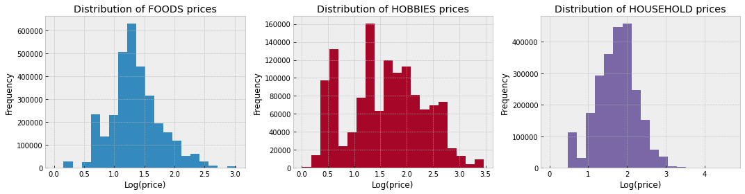
# Hobbiesは価格の分布が他に比べて大きい
sellp['Category'] = sellp['item_id'].str.split('_', expand=True)[0] # 複数の列に分割してpandas.DataFrameとして取得するには、引数expand=Trueを指定
fig, axs = plt.subplots(1, 3, figsize=(15, 4))
i = 0
for cat, d in sellp.groupby('Category'):
    # np.log1p:底をeとするa+1の対数を取る
    # 対数は0以下の計算ができないので、今回使用していると思われる(参考:https://www.sejuku.net/blog/70027)
    ax = d['sell_price'].apply(np.log1p) \
        .plot(kind='hist',
                         bins=20,
                         title=f'Distribution of {cat} prices',
                         ax=axs[i],
                                         color=next(color_cycle))
    ax.set_xlabel('Log(price)')
    i += 1
plt.tight_layout()

単純な予測
- 過去30日の平均売上を予測数値とする
# 最終日から30日の商品ごとの平均売上を算出
# to_dict()→商品idがキー、平均売上が値の辞書となる
thirty_day_avg_map = stv.set_index('id')[d_cols[-30:]].mean(axis=1).to_dict()
# F1-F28のリスト作成
fcols = [f for f in ss.columns if 'F' in f]
for f in fcols:
    # map関数?
    # ss[F○]に対応する値を入れる、これをforでF1-28繰り返して、提出ファイルができる
    ss[f] = ss['id'].map(thirty_day_avg_map).fillna(0)

ss.to_csv('submission.csv', index=False)
ss
| id | F1 | F2 | F3 | F4 | F5 | F6 | F7 | F8 | F9 | F10 | F11 | F12 | F13 | F14 | F15 | F16 | F17 | F18 | F19 | F20 | F21 | F22 | F23 | F24 | F25 | F26 | F27 | F28 | |
|---|---|---|---|---|---|---|---|---|---|---|---|---|---|---|---|---|---|---|---|---|---|---|---|---|---|---|---|---|---|
| 0 | HOBBIES_1_001_CA_1_validation | 0.966667 | 0.966667 | 0.966667 | 0.966667 | 0.966667 | 0.966667 | 0.966667 | 0.966667 | 0.966667 | 0.966667 | 0.966667 | 0.966667 | 0.966667 | 0.966667 | 0.966667 | 0.966667 | 0.966667 | 0.966667 | 0.966667 | 0.966667 | 0.966667 | 0.966667 | 0.966667 | 0.966667 | 0.966667 | 0.966667 | 0.966667 | 0.966667 |
| 1 | HOBBIES_1_002_CA_1_validation | 0.133333 | 0.133333 | 0.133333 | 0.133333 | 0.133333 | 0.133333 | 0.133333 | 0.133333 | 0.133333 | 0.133333 | 0.133333 | 0.133333 | 0.133333 | 0.133333 | 0.133333 | 0.133333 | 0.133333 | 0.133333 | 0.133333 | 0.133333 | 0.133333 | 0.133333 | 0.133333 | 0.133333 | 0.133333 | 0.133333 | 0.133333 | 0.133333 |
| 2 | HOBBIES_1_003_CA_1_validation | 0.566667 | 0.566667 | 0.566667 | 0.566667 | 0.566667 | 0.566667 | 0.566667 | 0.566667 | 0.566667 | 0.566667 | 0.566667 | 0.566667 | 0.566667 | 0.566667 | 0.566667 | 0.566667 | 0.566667 | 0.566667 | 0.566667 | 0.566667 | 0.566667 | 0.566667 | 0.566667 | 0.566667 | 0.566667 | 0.566667 | 0.566667 | 0.566667 |
| 3 | HOBBIES_1_004_CA_1_validation | 2.100000 | 2.100000 | 2.100000 | 2.100000 | 2.100000 | 2.100000 | 2.100000 | 2.100000 | 2.100000 | 2.100000 | 2.100000 | 2.100000 | 2.100000 | 2.100000 | 2.100000 | 2.100000 | 2.100000 | 2.100000 | 2.100000 | 2.100000 | 2.100000 | 2.100000 | 2.100000 | 2.100000 | 2.100000 | 2.100000 | 2.100000 | 2.100000 |
| 4 | HOBBIES_1_005_CA_1_validation | 1.266667 | 1.266667 | 1.266667 | 1.266667 | 1.266667 | 1.266667 | 1.266667 | 1.266667 | 1.266667 | 1.266667 | 1.266667 | 1.266667 | 1.266667 | 1.266667 | 1.266667 | 1.266667 | 1.266667 | 1.266667 | 1.266667 | 1.266667 | 1.266667 | 1.266667 | 1.266667 | 1.266667 | 1.266667 | 1.266667 | 1.266667 | 1.266667 |
| ... | ... | ... | ... | ... | ... | ... | ... | ... | ... | ... | ... | ... | ... | ... | ... | ... | ... | ... | ... | ... | ... | ... | ... | ... | ... | ... | ... | ... | ... |
| 60975 | FOODS_3_823_WI_3_evaluation | 0.000000 | 0.000000 | 0.000000 | 0.000000 | 0.000000 | 0.000000 | 0.000000 | 0.000000 | 0.000000 | 0.000000 | 0.000000 | 0.000000 | 0.000000 | 0.000000 | 0.000000 | 0.000000 | 0.000000 | 0.000000 | 0.000000 | 0.000000 | 0.000000 | 0.000000 | 0.000000 | 0.000000 | 0.000000 | 0.000000 | 0.000000 | 0.000000 |
| 60976 | FOODS_3_824_WI_3_evaluation | 0.000000 | 0.000000 | 0.000000 | 0.000000 | 0.000000 | 0.000000 | 0.000000 | 0.000000 | 0.000000 | 0.000000 | 0.000000 | 0.000000 | 0.000000 | 0.000000 | 0.000000 | 0.000000 | 0.000000 | 0.000000 | 0.000000 | 0.000000 | 0.000000 | 0.000000 | 0.000000 | 0.000000 | 0.000000 | 0.000000 | 0.000000 | 0.000000 |
| 60977 | FOODS_3_825_WI_3_evaluation | 0.000000 | 0.000000 | 0.000000 | 0.000000 | 0.000000 | 0.000000 | 0.000000 | 0.000000 | 0.000000 | 0.000000 | 0.000000 | 0.000000 | 0.000000 | 0.000000 | 0.000000 | 0.000000 | 0.000000 | 0.000000 | 0.000000 | 0.000000 | 0.000000 | 0.000000 | 0.000000 | 0.000000 | 0.000000 | 0.000000 | 0.000000 | 0.000000 |
| 60978 | FOODS_3_826_WI_3_evaluation | 0.000000 | 0.000000 | 0.000000 | 0.000000 | 0.000000 | 0.000000 | 0.000000 | 0.000000 | 0.000000 | 0.000000 | 0.000000 | 0.000000 | 0.000000 | 0.000000 | 0.000000 | 0.000000 | 0.000000 | 0.000000 | 0.000000 | 0.000000 | 0.000000 | 0.000000 | 0.000000 | 0.000000 | 0.000000 | 0.000000 | 0.000000 | 0.000000 |
| 60979 | FOODS_3_827_WI_3_evaluation | 0.000000 | 0.000000 | 0.000000 | 0.000000 | 0.000000 | 0.000000 | 0.000000 | 0.000000 | 0.000000 | 0.000000 | 0.000000 | 0.000000 | 0.000000 | 0.000000 | 0.000000 | 0.000000 | 0.000000 | 0.000000 | 0.000000 | 0.000000 | 0.000000 | 0.000000 | 0.000000 | 0.000000 | 0.000000 | 0.000000 | 0.000000 | 0.000000 |
60980 rows × 29 columns
kaggle walmart Prophet
Prophetを試す
lightGBMがぱっと思いつくが、Prophetも売上予測では有名で使いやすいので、kaggleのnotebookを試させて頂いた
使用したnotebook
https://www.kaggle.com/georsara1/fbprophet-try2-python-multiprocessing/execution
非常に参考になりました。ありがとうございます。
並列処理
処理時間を減らす為に並列処理を使用したようなことがコメントにかいてあったので、並列処理有りと無しで少量データで試したが、並列処理でない方が速度が速かった。
CPUとGPUも試したがCPUの方が速かった。
noteobookにCPUという記載があったので、元々GPUではなくCPUを使用する上で早くする想定なのかもしれないが、どちらでも並列処理でない方が速かった。
並列処理について全く理解できていないので理由は不明だがそのままやってみる。
結果
Public Score 0.78360と書いてある。
高い訳ではないが何もチューニングしていない。
Prophetは何も設定していない場合はデフォルトでトレンドやSeasonalityは考慮されているのだろうか。されてるんだろう。
考察
- イベント効果等何も触っていないのでまだまだできることはたくさんある
- 処理時間が長いのがネック
- 売上がマイナスで予測されることもあるようだ
次
- Prophetでも精度改善できるが、色々設定増やすと処理時間さらに長くなりそうなので次はlightgbmを試す
参考
並列処理について
- https://qiita.com/yukitaka13-1110/items/2580b4fc6c8a30d34661
- https://qiita.com/yukiB/items/203a6248c2d466b80d38
コード
インポート
```python
import pandas as pd
import numpy as np
from fbprophet import Prophet
from tqdm import tqdm, tnrange
from multiprocessing import Pool, cpu_count
```
データ読み込み
結果
```python
print(calendar_df.shape)
print(sales_train.shape)
print(sell_prices.shape)
print(submission.shape)
```
prophet関数定義
```python
def run_prophet(timeserie):
model = Prophet(uncertainty_samples=False) # 不確定区間(信頼区間)の計算をしない
model.fit(timeserie)
future = model.make_future_dataframe(periods=28, include_history=False)
forecast = model.predict(future)
return forecast
```
prophet実行
```python
start_from_ob = 800 # 795日目から学習(1119日間、3年くらい?)
for i in tnrange(sales_train.shape[0]): # 30490
# 1種類の商品の売上データ
temp_series = sales_train.iloc[i, start_from_ob:]
# インデックスを日付にする
temp_series.index = calendar_df["date"][start_from_ob:start_from_ob+len(temp_series)] # 2013/4/8-2016/4/30
temp_series = pd.DataFrame(temp_series)
temp_series = temp_series.reset_index()
# prophet用のカラム名に変更
temp_series.columns = ["ds", "y"]
# 並列処理
with Pool(cpu_count()) as p: # cpu_count()で最大実行可能コア数を取得
forecast1 = p.map(run_prophet, [temp_series]) # mapで関数を並列実行(run_prophetの引数を指定(temp_series))
# 提出ファイルに予測結果を入れる
submission.iloc[i, 1:] = forecast1[0]["yhat"].values
# 予測結果がマイナスの値を0に変換
submission.iloc[:, 1:][submission.iloc[:, 1:]<0]=0
# 提出ファイル保存
submission.to_csv("submission.csv", index=False)
```
